Galaxy morphometry
Primarily, morphometrics can be used to address galaxy morphology. Different works use a non-parametric approach to measure a galaxy’s shape characteristics. Lotz et al. (2004) characterize galaxies’ Concentration, Asymmetry. Furthermore, Ferrari et al. (2015) include Shannon entropy (information entropy) to quantify pixel values distribution. More recently, Rosa et al. (2018) characterized a galaxy’s morphology using the second moment of the gradient of the images through Gradient
Pattern Analysis. One of the critical features of non-parametric morphology estimation is understanding how a given parameter can reliably separate elliptical and spiral galaxies. Each metric measures patterns and forms in the image. Concentration (C) measures how tightly pixels are distributed in the galaxy structure, Asymmetry (A) measures irregularity of the form of the galaxy’s disk and bulge, Smoothness (S) measures the presence of the small structures in the galaxy’s disk (star-forming
regions), Entropy (H) is the measure of the heterogeneity of the pixel distribution and G2 analyses the asymmetric vector field (variation of flux intensity). When applied to an image with a clearly elliptical galaxy, usually, C will have high values, and A, S, H, and G2 will have low values. While in the case of a clearly spiral galaxy, it would be the opposite. Combining these values can provide a solid intuition of the class of unknown galaxies.
Besides using the morphometric parameters to study the actual physical processes molding galaxies directly, they can also be used in Machine Learning (ML) methods to discriminate ETGs from LTGs. Barchi et al. (2020) conducts a thorough study of ML using the CASHG2 system as the primary input information and galaxy Zoo 1, GZ1 (LINTOTT et al., 2008; LINTOTT et al., 2011) provides the “true” classification. These are the main ingredients for the training step. Several ML algorithms were
tested: Decision Tree (DT); Support Vector Machine (SVM); and Multilayer Perceptron (MLP). DT had a slightly better performance than the other two, with an overall accuracy (OA) of 98.5%, when dealing only with bright galaxies. When applying Deep Learning (DL) technique, they find only a tiny increase in OA, 99.5%.
CyMorph can also be applied to:
X-Ray map tracing gas from the ICM. By combining the results of the galaxy’s morphology and ICM hot gas X-Ray morphology properties, we plan to investigate how the cluster’s ICM morphological properties (high asymmetry, for example) affect member galaxies’ morphology.
Trace galaxy properties typical for \(\gamma\)-ray burst(GRB) hosts to prioritize targets with similar characteristics during gravitational wave optical follow-ups
(Santana-Silva et al. (in prep.).
In summary, CyMorph can extract five different metrics: Concentration (C), Asymmetry (A), Smoothness (S), Entropy (H), and Gradient Pattern Analysis (G2). Each of these metrics (except G2) ranges from 0 (min) to 1 (max) depending on the particular features of the content of the image. These metrics have a wide range of application in further resurch.
Metrics
Concentration
Concentration is straightforward to grasp intuitively; it simply measures how the flux is distributed on the galaxy profile, that is concentrated in the center (bulge) of the galaxy or distributed around the whole profile. The practical process to perform this kind of measurement consists of several steps. Literature has different approaches to calculate concentration (BERSHADY et al., 2000; GRAHAM et al., 2001b; ABRAHAM et al., 1994).. Here we fallow the method proposed in
Conselice (2003) and Lotz et al. (2004).
Figure 1 is showing the \(R_p\) and \(2*R_p\) (left panel) and \(\eta\) profile (left panel) of a spiral galaxy
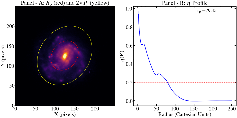
Figure 1
By definition, Concentration stands for a ratio of two portions of accumulated flux in two different fractions of the total flux of a galaxy. It is defined by: \(C = log_{10}(R_1/R_2)\), where \(R_1\) and \(R_2\) are the fractions of the total flux. They also called the outer and inner radii enclosing a fraction of total flux. The values of \(R_1\) and \(R_2\) can vary arbitrary, in range of 100 to 0 (containing all flux and none of it). Several studies used different pairs
of \(R_1\) and \(R_2\) (LOTZ et al., 2004; FERRARI et al., 2015).
Panel A in Figure 2 shows the accumulated flux curve for the elliptical galaxy, panel B for the spiral galaxy. From the comparison, it could be seen that flux growth in the case of the elliptical galaxy slows considerably already at \(R_2\), resulting in the highly concentrated center of this galaxy. In the case of a spiral galaxy, the accumulated flux keeps increasing more uniformly even after \(R_2\).
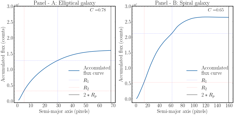
Figure 2
The processing starts by calculating the accumulated flux intensity curve and \(\eta\) profile on the cleaned image. Galaxies are resolved objects with poorly defined edges and do not all have the same radial surface brightness profile; some care is required to define the flux associated with each object. The \(\eta\) profile is necessary to obtain the Petrosian radius (\(R_p\)) because the total flux of a galaxy is defined by the accumulated flux until \(2*R_p\). The aperture
\(2*R_p\) is large enough to contain nearly all the flux for typical galaxy profiles but small enough that the sky noise impact is negligible Blanton et al. (2001). Based on the \(\eta\) profile, it is also largely insensitive to variations in the limiting surface brightness and redshift (in the sense of distance), providing reliable results for the galaxies with a high signal-to-noise ratio.
We follow Blanton et al. (2001) and Strateva et al. (2001) and set \(R_p\) on \(\eta = 0.2\) as it is shown in the right panel in Figure 1. The left panel in Figure 1 shows the portions in \(R_p\) and \(2*R_p\). Finally, it becomes possible to set the radii that contain the fractions of total flux. Intuitively and as it could be seen in the Figure 2, elliptical galaxies have the flux concentrated in the center, and it falls almost entirely in the R2 radius, leaving R1
with almost equal to R2 and pushing the ratio up. The opposite occurs with spiral galaxies, the main portion of the flux is concentrated in the center, but the spiral arms increase the total flux located in R2 and drive the ratio down.
Asymmetry
Asymmetry could be the most uncomplicated metric to extract, and the simplicity consists in the fact that it is not necessary to perform any additional operation on the \(segmented\_image\). Tracing the asymmetry distribution in the galaxy profile can help to reveal dynamic processes in galaxies. This is especially true when we talk about collisionless stars and can track the matter distribution more precisely. For instance, galaxies disturbed by interactions or mergers with another galaxy
will tend to have high asymmetries (CONSELICE et al., 2000).
Asymmetry, by definition, measures the degree of irregularity of the galaxy profile. To obtain it, CyMorph will rotate the segmented image by \(180^{\circ}\) and run a \(for\) loop on both of the images (segmented and rotated). This loop will compare each \([i,j]\) pixel of both of the images, and in case if both are not zero (containing flux counts), the non-zero pixels will be stored in \(list1\) and \(list2\)—these lists of pixels for segmented and rotated images, respectively.
Figure 3 is showing how does correlation works when we collect the pixels on input (Panel A) and rotated (Panel B) images. Panel C shows the visual correlation of \(list1\) and \(list2\), rotated and original pixels respectively.
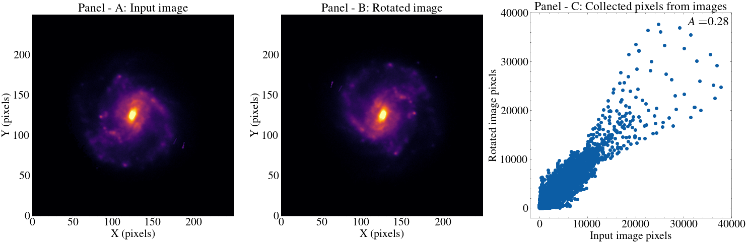
Figure 3
The next step would be the calculation of the correlation coefficient between the segmented image and the rotated image pixels lists. CyMorph will use Pearson and Spearman Ranks (PRESS,2005) coefficient functions to calculate the correlation coefficients between the two lists. In the case of an elliptical galaxy, the correlation coefficient will be high since the pixels of the elliptical galaxy are fairly heterogeneously distributed. In the case of a spiral galaxy, where pixels have a much
higher gradient, it will mean that, after rotation, two pixels on the same position will have very different values. The formula to calculate A is \(A = 1 - spearmanr(list1, list2)\). When the correlation coefficient is high (meaning that there is no significant difference between pixel values on both images), asymmetry will be low (case of an elliptical galaxy). In case if the correlation coefficient is low, the asymmetry will be high (case of spiral galaxy).
As it could be seen in Figure 3, if one rotates a spiral galaxy, the correlation would be low since spiral arms and similar irregularities will contribute to the fact that the same pixels would have very different flux values. It would be the opposite if we rotated the elliptical one. The reason is that elliptical galaxies have nearly perfect flux distribution. So the correlation will be high.
Smoothness
Smoothness (or clumpiness) is calculated very similarly with asymmetry. It calculates the Pearson and Spearman ranks correlation coefficients between the segmented image and its smoothed version (ABRAHAM et al., 1996; CONSELICE, 2003; FERRARI et al., 2015). Instead of rotation, we are applying a second order of the Butter filter to smooth the original image. This filter provides the advantage of continuous adaptive control of the smoothing degree applied to the image
(KASZYNSKI; PISKOROWSKI, 2006; PEDRINI; SCHWARTZ, 2008; SAUTTER, 2018). By intuition, if one tries to smooth the elliptical galaxy, the result will be almost the same image because naturally, these galaxies are smooth. Scanning the images, storing the pixels to lists, and calculating the coefficient will result in a high correlation between the segmented and smoothed image. Spiral galaxies will produce the opposite result, for the correlation will be low between the images, and clumpiness
will be high. The formula to obtain S is \(S = 1 - spearmanr(list1, list2)\).
The nomenclature could bring confusion, but the logic behind this metric consists in the fact that spiral galaxies will present small structures inside the disk that will contribute to the high Clumpiness values, while elliptical galaxies, naturally smooth, will have high correlation and low Clumpiness value.
From Figure 4 we can see that smoothing the spiral galaxy produces a significant difference. In the case of an elliptical galaxy, it would be almost unnoticeable. The level of change in the image after the smoothing is the key factor in the metric calculation. Figure 4 is showing how does correlation works when we collect the pixels on input and smoothed image. Panel C is showing the visual correlation of \(list1\) and \(list2\), rotated and original pixels respectively.
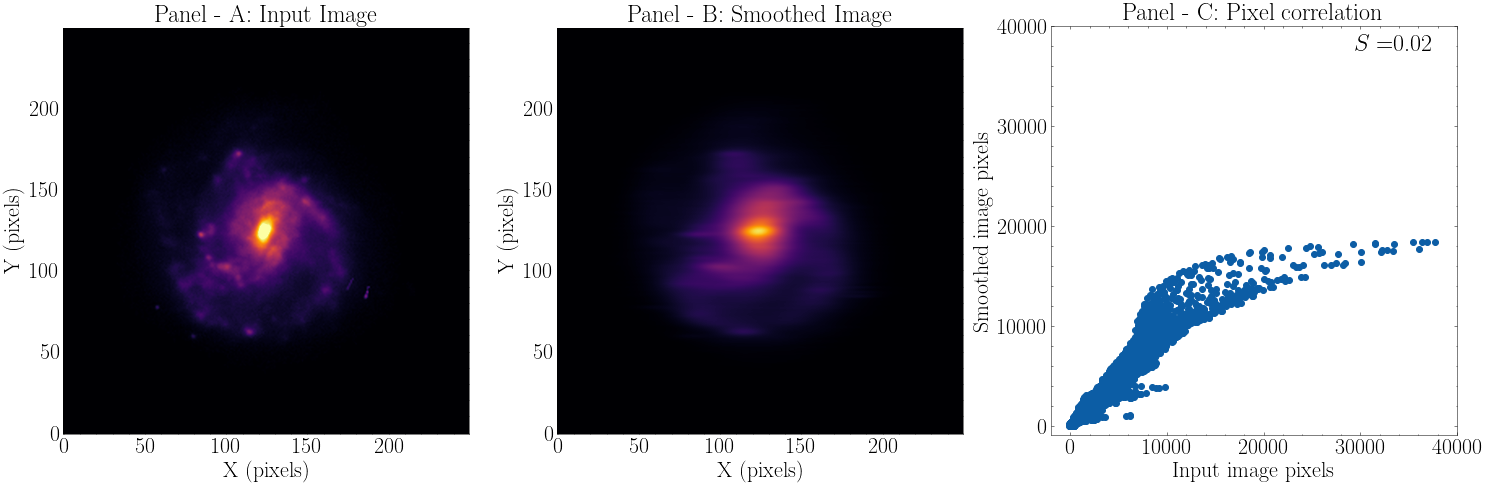
Figure 4
Entropy
Entropy (H) works very similarly to the concentration in the sense that it measures pixel density/frequency in a given number of bins. Entropy bins number is a parameter that can be tuned to adapt better to the data at hand, and it is responsible for how many bins the flux distribution will be split. In a simplified manner, H measures the distribution of pixel values in the image by dividing the image in an arbitrary number of bins. The process of the H extraction does not have any additional image manipulation. The input image pixels are raveled (converted to 1d array) and are used to calculate values of the histogram (frequency of the flux) and bin edges with \(numpy.histogram\). The illustration of this process is shown in Figure 5.
It is worth noting how the flux of the elliptical galaxy is concentrated in a small area, while the spiral galaxy’s flux occupies a broader area of flux distribution. The next step is the normalization of the frequency counts by maximum count and then calculating the entropy value with:
\begin{equation} H(I)=-\sum_{k}^{K} p\left(I_{k}\right) \log \left[p\left(I_{k}\right)\right] \end{equation}
Equation 1
where:
\(p(I_{k})\) - s the probability of occurrence of the value \(I_{k}\)
\(K\) - number of bins that data was split
For discrete variables, \(H\) reaches the maximum value for a uniform distribution, when \(p(I_{k}) = 1/K\) for all \(k\), resulting in \(H_{max} = \log K\). The minimum entropy is that of a delta function, for which \(H = 0\). Hence, we can get the normalized entropy with:
\begin{equation} \widetilde{H}(I)=\frac{H(I)}{H_{\max }} \quad 0 \leqslant \widetilde{H}(I) \leqslant 1 \end{equation}
Equation 2
Elliptical galaxies are expected to have low entropy (for having natural homogeneity of flux (pixel value) distribution), and spiral galaxies are expected to have high values of entropy (by presenting irregular structures and those having pixel value heterogeneity naturally) (BISHIP, 2007; FERRARI et al., 2015).
The top row in the Figure 5 shows the flux distribution of an elliptical galaxy when the image is raveled and used as input for the \(numpy.histogram\). The thin distribution limited to low counts with a fast decrease slope characterizes the flux concentration of the elliptical profile. We can see the opposite in the case of a spiral galaxy (middle row), where the flux is spread over a bigger area of the flux axis.
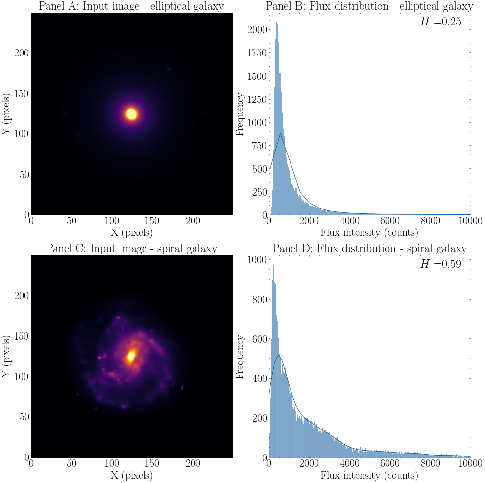
Figure 5
Gradient Pattern Analysis (second moment)
The second moment of Gradient Pattern Analysis (GPA), in short G2, can be considered the most complex metric to be calculated. According to Sautter (2018), GPA has four moments, but for the galaxy morphology classification, only the first and second are currently used. Rosa et al. (2018) showed that improved and revised version of the second moment (with due modifications) shows best results in galaxy separations when compared with classic CAS classification (CONSELICE, 2003). We
have performed a revision and optimization of the code to comply with the original definition.
Extraction process
The first step is to convert all zeros in the image to \(numpy.nan\). This condition assures that the border pixels of the image will be ignored during the gradient field generation. Otherwise, they would contribute detrimentally to the final result. Then we are generating the gradient field with \(numpy.gradient(segmented\_image)\).
In the next step, we will generate an asymmetric gradient field. This process consists of locating pairs of pixels located at the same distance from the center and comparing modulus (strength) and phase (direction) between them. If two pixels of the given pair have the same modulus but opposite phases, they will be considered symmetric and removed. This process will be performed on all the unique pairs of pixels (to exclude the repetition). The resulting lattice is called an asymmetry vector field because all symmetric pairs are removed. Next, we will obtain the count of asymmetric vectors, their sum, and their modulus sum. To determine if the vectors are aligned and have the same magnitude, we need to calculate \(confluence\) using the equation 3:
\begin{equation} confluence = \left(\frac{\left|\sum_{i}^{V_{a}} v_{a}^{i}\right|}{\sum_{i}^{V_{a}}\left|v_{a}^{i}\right|}\right) \end{equation}
Equation 3
where:
\(v_{a}\) - list of asymmetrical vectors
\(V_{A}\) - count of asymmetric vectors
The final calculation of G2 value is obtained by the equation 4 (ROSA et al., 1999; RAMOS et al., 2000; ROSA et al., 2003; SAUTTER, 2018):
\begin{equation} G_{2} = \frac{V_{A}} {V - V_{c}} (2-confluence) \end{equation}
Equation 4
where:
\(V_{A}\) - total valid pixels
\(V_{c}\) - contour pixels
\(V_{A}\) - asymmetric pixels
\(2\) - normalization factor
Figure 6 shows results in two fringe cases: random noise, resulting in maximum G2 value (as there are very few pairs that end up canceled) and Gaussian noise, resulting in minimum G2 value (as there are all pixel pairs end up canceled).
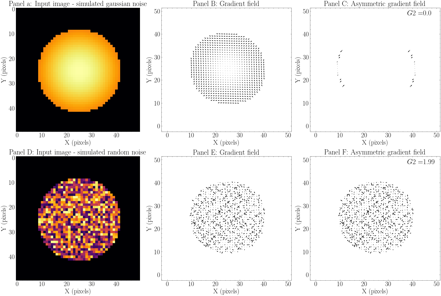
Figure 6
It is possible to perform fine-tuning of the G2. It has two tolerances: \(modulus\_tolerance\). \(modulus\_tolerance\) is responsible for serving as the threshold of the minimum acceptable strength difference between two vectors. Worth noting that modulus are normalized by the maximum value during the calculation, so the \(modulus\_tolerance\) can be influential even with low values, as it ranges from 0 (no tolerance at all) to 1 (any two pixels are considered to have same modulus). \(phase\_tolerance\) serves as a threshold of minimal acceptable angle difference between two pixels (their vectors). It ranges from 0 (no tolerance) to 3.14 (any any two pixels are considered to have same angle)
The top row in Figure 6 shows the results expected with a simulated input image with Gaussian noise. In this case, almost all the vectors should cancel out, the asymmetric gradient field should be empty, and the resulting value of G2 should be near to 0 (minimum value of G2). The bottom row shows the results expected with a simulated input image with random noise. In this case, almost all the vectors will be preserved, and the resulting value of G2 should be near to 2.0 (maximum value of G2).
Intuitively, elliptical galaxies will have a lot of the same vectors, being naturally smooth and round, and as a consequence, many vectors will be canceled. In the case of spiral galaxies, the internal structures distort the gradient field, resulting in many vectors being preserved. Figure 7 shows visualization of this behavior.
The top row shows the results expected with elliptical galaxies. Generally, most of the vectors should cancel out, resulting in a low value of G2 (\(G2 < 0.5\)). The bottom row shows the results expected with spiral galaxies. In this case, most of the vectors will be preserved, and the resulting value of G2 should be high (\(G2 > 1.5\)).
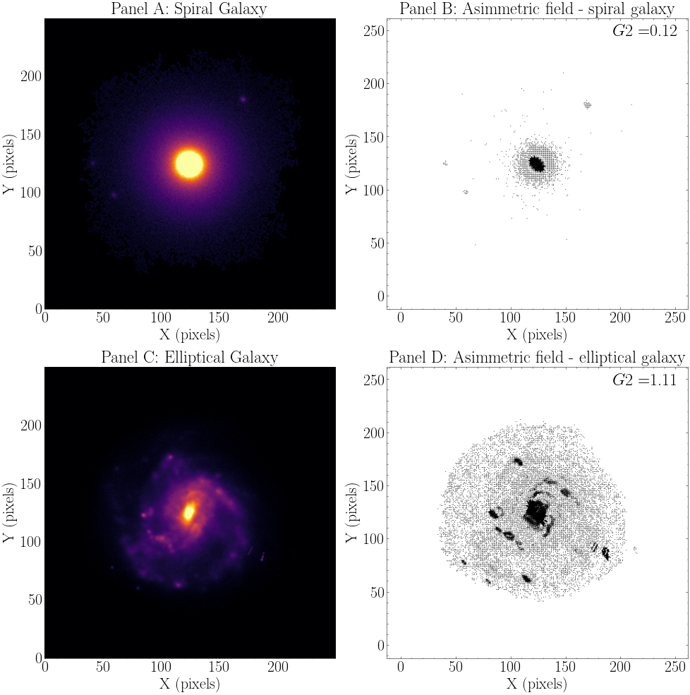
Figure 7